Analysing biotic communities
The previous tutorial covered a bunch of the basics with some pretty straightforward data, and was more focused on how R works. Now we’ll be looking at slightly more complicated data (species data), which will require learning some fancier data handling.
R has a ridiculous number of libraries and functions for analyzing environmental and biodiversity data - check out the
Environmetrics Task View for a primer on a small sample. The issue is that many of them have their own specific data format requirements, requiring an inordinate amount of data wrangling. My aim for this session is to walk you through an example dataset, sharing a few tidyverse and base R data wrangling tricks, and highlighting some common perils and pitfalls when analysing patterns and change in biotic community survey data.
First, let’s get the R packages we need and set our working directory
library(tidyverse)
library(readxl)
library(vegan) #comment out with "#" if you don't have this installed - or run install.packages("vegan")

setwd("/home/jasper/GIT/academic-kickstart/static/datasets/")
#Change to your local path to the folder where you put the dataset
Description of community data
We’re going to use the same dataset from Slingsby et al. 2017 that we used in the previous tutorial. The data can be downloaded here. It’s a ~10MB .xlsx file.
This is a vegetation survey of 81 plots, each 5 by 10m, from across the Cape of Good Hope section of Table Mountain National Park. For more information check out the worksheet labeled METADATA and/or read the paper.
Let’s look at the sheets in our Excel workbook.
excel_sheets("pnas.1619014114.sd01.xlsx")
##  [1] "METADATA"           "weather"            "fires"
##  [4] "postfireweather"    "enviroment"         "excluded_spp"
##  [7] "veg1966"            "veg1996"            "veg2010"
## [10] "traits"             "speciesclimatedata"
There’s quite a few sheets in the workbook, but the datasets most commonly used in analyses of biotic communities are three separate data objects (usually matrices, but see below) that include:
- Species by sites - also called the community data matrix (where values are one of presence/absence, counts/abundance, %cover, biomass or similar
- Environmental variables by site (e.g. soils, climate, location, etc)
- Traits by species (e.g. growth form or other qualitative or quantitative life history or functional traits)
We have environment and traits, which are the second and third matrices, and in this case we have three community matrices (veg1966, veg1996 and veg2010), because the sites were first surveyed in 1966 and then resurveyed in 1996 and 2010.
Note that if you ever want to see what data are in a sheet, but don’t want to open the file in Excel, you can easily have a glimpse at them to by just selecting a small range in read_excel() like so
read_excel("pnas.1619014114.sd01.xlsx", sheet = "veg1966", range = "A1:K5")
## New names:
## * `` -> ...1
## # A tibble: 4 x 11
##   ...1  `Adenandra unif… `Adenandra vill… `Adenocline pau… `Agathosma cili…
##   <chr>            <dbl>            <dbl>            <dbl>            <dbl>
## 1 CP_1                 0                7                0                0
## 2 CP_10                0                0                0                0
## 3 CP_1…                0                7                0                0
## 4 CP_12                0                0                0                0
## # … with 6 more variables: `Agathosma hookeri` <dbl>, `Agathosma
## #   imbricata` <dbl>, `Agathosma lanceolata` <dbl>, `Agathosma
## #   serpyllacea` <dbl>, `Aizoon paniculatum` <dbl>, `Amphithalea
## #   ericifolia` <dbl>
read_excel("pnas.1619014114.sd01.xlsx", sheet = "veg2010", range = "A1:K5")
## New names:
## * `` -> ...1
## # A tibble: 4 x 11
##   ...1  `Acacia saligna` `Adenandra unif… `Adenandra vill… `Agapanthus wal…
##   <chr>            <dbl>            <dbl>            <dbl>            <dbl>
## 1 CP_1                 0                0                3                0
## 2 CP_10                0                0                0                0
## 3 CP_12                0                0                0                0
## 4 CP_13                0                0                0                0
## # … with 6 more variables: `Agathosma ciliaris` <dbl>, `Agathosma
## #   hookeri` <dbl>, `Agathosma imbricata` <dbl>, `Agathosma serpyllacea` <dbl>,
## #   `Albuca flaccida` <dbl>, `Albuca juncifolia` <dbl>
In this case the veg1966 and veg1996 data were Braun-Blanquet cover-abundance classes, which I have converted to abundance using the midpoint of each class. THIS IS NOT NECESSARILY DEFENSIBLE!!! but it’s fine for the purposes of this tutorial. The veg2010 dataset is actual counts of individuals.
Let’s read them in and have a closer look.
species66 <- read_excel("pnas.1619014114.sd01.xlsx", sheet = "veg1966")
## New names:
## * `` -> ...1
head(species66)
## # A tibble: 6 x 428
##   ...1  `Adenandra unif… `Adenandra vill… `Adenocline pau… `Agathosma cili…
##   <chr>            <dbl>            <dbl>            <dbl>            <dbl>
## 1 CP_1                 0                7                0                0
## 2 CP_10                0                0                0                0
## 3 CP_1…                0                7                0                0
## 4 CP_12                0                0                0                0
## 5 CP_13                0                0                0                0
## 6 CP_14                0                0                0                0
## # … with 423 more variables: `Agathosma hookeri` <dbl>, `Agathosma
## #   imbricata` <dbl>, `Agathosma lanceolata` <dbl>, `Agathosma
## #   serpyllacea` <dbl>, `Aizoon paniculatum` <dbl>, `Amphithalea
## #   ericifolia` <dbl>, `Anaxeton laeve` <dbl>, `Anemone knowltonia` <dbl>,
## #   `Anthochortus laxiflorus` <dbl>, `Anthospermum aethiopicum` <dbl>,
## #   `Anthospermum bergianum` <dbl>, `Anthospermum galioides` <dbl>, `Apium
## #   decumbens` <dbl>, `Arctotis aspera` <dbl>, `Argyrolobium filiforme` <dbl>,
## #   `Aristea africana` <dbl>, `Aristea capitata` <dbl>, `Aristea glauca` <dbl>,
## #   `Aspalathus abietina` <dbl>, `Aspalathus argyrella` <dbl>, `Aspalathus
## #   callosa` <dbl>, `Aspalathus capensis` <dbl>, `Aspalathus carnosa` <dbl>,
## #   `Aspalathus chenopoda` <dbl>, `Aspalathus divaricata` <dbl>, `Aspalathus
## #   ericifolia` <dbl>, `Aspalathus hispida` <dbl>, `Aspalathus
## #   laricifolia` <dbl>, `Aspalathus linguiloba` <dbl>, `Aspalathus
## #   microphylla` <dbl>, `Aspalathus retroflexa` <dbl>, `Aspalathus
## #   sericea` <dbl>, `Aspalathus serpens` <dbl>, `Asparagus aethiopicus` <dbl>,
## #   `Asparagus capensis` <dbl>, `Asparagus lignosus` <dbl>, `Asparagus
## #   rubicundus` <dbl>, `Berkheya barbata` <dbl>, `Berzelia abrotanoides` <dbl>,
## #   `Berzelia lanuginosa` <dbl>, `Bobartia filiformis` <dbl>, `Bobartia
## #   gladiata` <dbl>, `Bobartia indica` <dbl>, `Bolusafra bituminosa` <dbl>,
## #   `Bulbine abyssinica` <dbl>, `Caesia contorta` <dbl>, `Capelio
## #   tabularis` <dbl>, `Capeobolus brevicaulis` <dbl>, `Capeochloa
## #   cincta` <dbl>, `Carpacoce spermacocea` <dbl>, `Carpacoce
## #   vaginellata` <dbl>, `Carpobrotus acinaciformis` <dbl>, `Cassine
## #   peragua` <dbl>, `Cassytha ciliolata` <dbl>, `Centella affinis` <dbl>,
## #   `Centella glabrata` <dbl>, `Centella macrocarpa` <dbl>, `Centella
## #   tridentata` <dbl>, `Chironia baccifera` <dbl>, `Chironia decumbens` <dbl>,
## #   `Chironia linoides` <dbl>, `Chrysocoma coma-aurea` <dbl>, `Cineraria
## #   geifolia` <dbl>, `Cliffortia atrata` <dbl>, `Cliffortia falcata` <dbl>,
## #   `Cliffortia ferruginea` <dbl>, `Cliffortia filifolia` <dbl>, `Cliffortia
## #   glauca` <dbl>, `Cliffortia obcordata` <dbl>, `Cliffortia
## #   polygonifolia` <dbl>, `Cliffortia ruscifolia` <dbl>, `Cliffortia
## #   stricta` <dbl>, `Cliffortia subsetacea` <dbl>, `Clutia alaternoides` <dbl>,
## #   `Clutia ericoides` <dbl>, `Clutia polygonoides` <dbl>, `Coleonema
## #   album` <dbl>, `Conyza pinnatifida` <dbl>, `Corymbium africanum` <dbl>,
## #   `Corymbium glabrum` <dbl>, `Crassula capensis` <dbl>, `Crassula
## #   coccinea` <dbl>, `Crassula cymosa` <dbl>, `Crassula fascicularis` <dbl>,
## #   `Crassula flava` <dbl>, `Crassula nudicaulis` <dbl>, `Crassula
## #   subulata` <dbl>, `Cullumia squarrosa` <dbl>, `Cussonia thyrsiflora` <dbl>,
## #   `Cymbopogon marginatus` <dbl>, `Cynanchum africanum` <dbl>, `Cynanchum
## #   obtusifolium` <dbl>, `Cynodon dactylon` <dbl>, `Cyperus thunbergii` <dbl>,
## #   `Diastella divaricata` <dbl>, `Dilatris corymbosa` <dbl>, `Dilatris
## #   pillansii` <dbl>, `Dimorphotheca nudicaulis` <dbl>, `Diosma hirsuta` <dbl>,
## #   `Diosma oppositifolia` <dbl>, …
species10 <- read_excel("pnas.1619014114.sd01.xlsx", sheet = "veg2010")
## New names:
## * `` -> ...1
head(species10)
## # A tibble: 6 x 339
##   ...1  `Acacia saligna` `Adenandra unif… `Adenandra vill… `Agapanthus wal…
##   <chr>            <dbl>            <dbl>            <dbl>            <dbl>
## 1 CP_1                 0                0                3                0
## 2 CP_10                0                0                0                0
## 3 CP_12                0                0                0                0
## 4 CP_13                0                0                0                0
## 5 CP_14                0                0                0                0
## 6 CP_15                0                0                0                0
## # … with 334 more variables: `Agathosma ciliaris` <dbl>, `Agathosma
## #   hookeri` <dbl>, `Agathosma imbricata` <dbl>, `Agathosma serpyllacea` <dbl>,
## #   `Albuca flaccida` <dbl>, `Albuca juncifolia` <dbl>, `Amphithalea
## #   ericifolia` <dbl>, `Anaxeton laeve` <dbl>, `Anemone knowltonia` <dbl>,
## #   `Anthochortus capensis` <dbl>, `Anthospermum aethiopicum` <dbl>,
## #   `Anthospermum bergianum` <dbl>, `Anthospermum galioides` <dbl>, `Apium
## #   decumbens` <dbl>, `Arctotheca calendula` <dbl>, `Aristea africana` <dbl>,
## #   `Aspalathus callosa` <dbl>, `Aspalathus capensis` <dbl>, `Aspalathus
## #   carnosa` <dbl>, `Aspalathus chenopoda` <dbl>, `Aspalathus ciliaris` <dbl>,
## #   `Aspalathus hispida` <dbl>, `Aspalathus linguiloba` <dbl>, `Aspalathus
## #   microphylla` <dbl>, `Aspalathus retroflexa` <dbl>, `Aspalathus
## #   serpens` <dbl>, `Asparagus capensis` <dbl>, `Asparagus lignosus` <dbl>,
## #   `Asparagus rubicundus` <dbl>, `Babiana ambigua` <dbl>, `Babiana
## #   villosula` <dbl>, `Berkheya barbata` <dbl>, `Berzelia abrotanoides` <dbl>,
## #   `Berzelia lanuginosa` <dbl>, `Bobartia gladiata` <dbl>, `Bobartia
## #   indica` <dbl>, `Bolusafra bituminosa` <dbl>, `Bulbine abyssinica` <dbl>,
## #   `Bulbine alooides` <dbl>, `Bulbine lagopus` <dbl>, `Caesia contorta` <dbl>,
## #   `Capelio tabularis` <dbl>, `Capeochloa cincta` <dbl>, `Carpobrotus
## #   acinaciformis` <dbl>, `Carpobrotus edulis` <dbl>, `Cassine peragua` <dbl>,
## #   `Cassytha ciliolata` <dbl>, `Centella macrocarpa` <dbl>, `Centella
## #   tridentata` <dbl>, `Chenolea diffusa` <dbl>, `Chironia baccifera` <dbl>,
## #   `Chironia decumbens` <dbl>, `Chironia linoides` <dbl>, `Cliffortia
## #   atrata` <dbl>, `Cliffortia falcata` <dbl>, `Cliffortia ferruginea` <dbl>,
## #   `Cliffortia obcordata` <dbl>, `Cliffortia stricta` <dbl>, `Cliffortia
## #   subsetacea` <dbl>, `Clutia alaternoides` <dbl>, `Clutia ericoides` <dbl>,
## #   `Coleonema album` <dbl>, `Colpoon compressum` <dbl>, `Corymbium
## #   africanum` <dbl>, `Corymbium glabrum` <dbl>, `Cotula coronopifolia` <dbl>,
## #   `Cotula turbinata` <dbl>, `Crassula fascicularis` <dbl>, `Crassula
## #   nudicaulis` <dbl>, `Cymbopogon marginatus` <dbl>, `Cynodon dactylon` <dbl>,
## #   `Dasispermum hispidum` <dbl>, `Diastella divaricata` <dbl>, `Dilatris
## #   pillansii` <dbl>, `Diosma hirsuta` <dbl>, `Diosma oppositifolia` <dbl>,
## #   `Diospyros glabra` <dbl>, `Disa bracteata` <dbl>, `Disa obliqua` <dbl>,
## #   `Disa purpurascens` <dbl>, `Disparago tortilis` <dbl>, `Disperis
## #   capensis` <dbl>, `Drimia capensis` <dbl>, `Drosanthemum candens` <dbl>,
## #   `Drosera aliciae` <dbl>, `Drosera trinervia` <dbl>, `Edmondia
## #   sesamoides` <dbl>, `Ehrharta calycina` <dbl>, `Ehrharta ramosa` <dbl>,
## #   `Elegia cuspidata` <dbl>, `Elegia filacea` <dbl>, `Elegia juncea` <dbl>,
## #   `Elegia microcarpa` <dbl>, `Elegia nuda` <dbl>, `Elegia persistens` <dbl>,
## #   `Elegia stipularis` <dbl>, `Elegia vaginulata` <dbl>, `Elytropappus
## #   scaber` <dbl>, `Eragrostis capensis` <dbl>, `Erepsia anceps` <dbl>, …
Yup, that looks about right.
We’re going to start playing with the 1966 data in a second, but first, what if your data aren’t in a species by site matrix?
Often biodiversity data are stored in “long” or “list” format with three columns like Site, Species and Abundance or similar. This is also the tidy data format preferred by the various packages that adopt a tidyverse approach, so it is worth taking a second to explore a few tricks that help convert between formats.
In our case we have the data in matrix format, so first let’s convert it to long format.
hmm <- species66 %>% pivot_longer(cols = -1,
                                  names_to = "Species",
                                  values_to = "Abundance")

hmm
## # A tibble: 34,587 x 3
##    ...1  Species                Abundance
##    <chr> <chr>                      <dbl>
##  1 CP_1  Adenandra uniflora             0
##  2 CP_1  Adenandra villosa              7
##  3 CP_1  Adenocline pauciflora          0
##  4 CP_1  Agathosma ciliaris             0
##  5 CP_1  Agathosma hookeri              0
##  6 CP_1  Agathosma imbricata            0
##  7 CP_1  Agathosma lanceolata           0
##  8 CP_1  Agathosma serpyllacea          0
##  9 CP_1  Aizoon paniculatum             0
## 10 CP_1  Amphithalea ericifolia         2
## # … with 34,577 more rows
Note that the names_to command sets a name for the column where the column names from the matrix are stored, while ‘values_to’ names the value column. You also have to select the columns you want to gather, and in this case we wanted to exclude the first column (the sites) as they are not abundance data.
Now let’s convert the long format data back to a matrix.
hmm <- hmm %>% pivot_wider(id_cols = 1,
                           names_from = Species,
                           values_from = Abundance,
                           values_fill = 0)

hmm
## # A tibble: 81 x 428
##    ...1  `Adenandra unif… `Adenandra vill… `Adenocline pau… `Agathosma cili…
##    <chr>            <dbl>            <dbl>            <dbl>            <dbl>
##  1 CP_1                 0                7                0                0
##  2 CP_10                0                0                0                0
##  3 CP_1…                0                7                0                0
##  4 CP_12                0                0                0                0
##  5 CP_13                0                0                0                0
##  6 CP_14                0                0                0                0
##  7 CP_15                0                7                0                0
##  8 CP_16                0                0                0                0
##  9 CP_17                0                0                0                0
## 10 CP_18                0                0                0                0
## # … with 71 more rows, and 423 more variables: `Agathosma hookeri` <dbl>,
## #   `Agathosma imbricata` <dbl>, `Agathosma lanceolata` <dbl>, `Agathosma
## #   serpyllacea` <dbl>, `Aizoon paniculatum` <dbl>, `Amphithalea
## #   ericifolia` <dbl>, `Anaxeton laeve` <dbl>, `Anemone knowltonia` <dbl>,
## #   `Anthochortus laxiflorus` <dbl>, `Anthospermum aethiopicum` <dbl>,
## #   `Anthospermum bergianum` <dbl>, `Anthospermum galioides` <dbl>, `Apium
## #   decumbens` <dbl>, `Arctotis aspera` <dbl>, `Argyrolobium filiforme` <dbl>,
## #   `Aristea africana` <dbl>, `Aristea capitata` <dbl>, `Aristea glauca` <dbl>,
## #   `Aspalathus abietina` <dbl>, `Aspalathus argyrella` <dbl>, `Aspalathus
## #   callosa` <dbl>, `Aspalathus capensis` <dbl>, `Aspalathus carnosa` <dbl>,
## #   `Aspalathus chenopoda` <dbl>, `Aspalathus divaricata` <dbl>, `Aspalathus
## #   ericifolia` <dbl>, `Aspalathus hispida` <dbl>, `Aspalathus
## #   laricifolia` <dbl>, `Aspalathus linguiloba` <dbl>, `Aspalathus
## #   microphylla` <dbl>, `Aspalathus retroflexa` <dbl>, `Aspalathus
## #   sericea` <dbl>, `Aspalathus serpens` <dbl>, `Asparagus aethiopicus` <dbl>,
## #   `Asparagus capensis` <dbl>, `Asparagus lignosus` <dbl>, `Asparagus
## #   rubicundus` <dbl>, `Berkheya barbata` <dbl>, `Berzelia abrotanoides` <dbl>,
## #   `Berzelia lanuginosa` <dbl>, `Bobartia filiformis` <dbl>, `Bobartia
## #   gladiata` <dbl>, `Bobartia indica` <dbl>, `Bolusafra bituminosa` <dbl>,
## #   `Bulbine abyssinica` <dbl>, `Caesia contorta` <dbl>, `Capelio
## #   tabularis` <dbl>, `Capeobolus brevicaulis` <dbl>, `Capeochloa
## #   cincta` <dbl>, `Carpacoce spermacocea` <dbl>, `Carpacoce
## #   vaginellata` <dbl>, `Carpobrotus acinaciformis` <dbl>, `Cassine
## #   peragua` <dbl>, `Cassytha ciliolata` <dbl>, `Centella affinis` <dbl>,
## #   `Centella glabrata` <dbl>, `Centella macrocarpa` <dbl>, `Centella
## #   tridentata` <dbl>, `Chironia baccifera` <dbl>, `Chironia decumbens` <dbl>,
## #   `Chironia linoides` <dbl>, `Chrysocoma coma-aurea` <dbl>, `Cineraria
## #   geifolia` <dbl>, `Cliffortia atrata` <dbl>, `Cliffortia falcata` <dbl>,
## #   `Cliffortia ferruginea` <dbl>, `Cliffortia filifolia` <dbl>, `Cliffortia
## #   glauca` <dbl>, `Cliffortia obcordata` <dbl>, `Cliffortia
## #   polygonifolia` <dbl>, `Cliffortia ruscifolia` <dbl>, `Cliffortia
## #   stricta` <dbl>, `Cliffortia subsetacea` <dbl>, `Clutia alaternoides` <dbl>,
## #   `Clutia ericoides` <dbl>, `Clutia polygonoides` <dbl>, `Coleonema
## #   album` <dbl>, `Conyza pinnatifida` <dbl>, `Corymbium africanum` <dbl>,
## #   `Corymbium glabrum` <dbl>, `Crassula capensis` <dbl>, `Crassula
## #   coccinea` <dbl>, `Crassula cymosa` <dbl>, `Crassula fascicularis` <dbl>,
## #   `Crassula flava` <dbl>, `Crassula nudicaulis` <dbl>, `Crassula
## #   subulata` <dbl>, `Cullumia squarrosa` <dbl>, `Cussonia thyrsiflora` <dbl>,
## #   `Cymbopogon marginatus` <dbl>, `Cynanchum africanum` <dbl>, `Cynanchum
## #   obtusifolium` <dbl>, `Cynodon dactylon` <dbl>, `Cyperus thunbergii` <dbl>,
## #   `Diastella divaricata` <dbl>, `Dilatris corymbosa` <dbl>, `Dilatris
## #   pillansii` <dbl>, `Dimorphotheca nudicaulis` <dbl>, `Diosma hirsuta` <dbl>,
## #   `Diosma oppositifolia` <dbl>, …
Note that I added the values_fill = 0 command, because a major advantage of long format biodiversity data is you don’t usually retain records of species with zero abundance at a site (i.e. absences) as these are usually implicit. They do need to be present in a matrix, so this command simply tells the function to fill absence records with 0.
Is the output the same as our original data?
identical(hmm, species66)
## [1] TRUE
Ok, so what do we want to know?
Summarizing community data
Total abundance by plot? We can do this by summing the abundance of all species in each site (i.e. row in the matrix).
rowSums(species66)
## Error in rowSums(species66): 'x' must be numeric
A classic R error message. It seems unhelpful, but as you learn R the error messages make more sense. In this case it is telling us that not all the values in species66 are numbers (i.e. of class “numeric”). Some may be of class “character”, “factor”, etc.
If we look at the data more closely…
head(species66)
## # A tibble: 6 x 428
##   ...1  `Adenandra unif… `Adenandra vill… `Adenocline pau… `Agathosma cili…
##   <chr>            <dbl>            <dbl>            <dbl>            <dbl>
## 1 CP_1                 0                7                0                0
## 2 CP_10                0                0                0                0
## 3 CP_1…                0                7                0                0
## 4 CP_12                0                0                0                0
## 5 CP_13                0                0                0                0
## 6 CP_14                0                0                0                0
## # … with 423 more variables: `Agathosma hookeri` <dbl>, `Agathosma
## #   imbricata` <dbl>, `Agathosma lanceolata` <dbl>, `Agathosma
## #   serpyllacea` <dbl>, `Aizoon paniculatum` <dbl>, `Amphithalea
## #   ericifolia` <dbl>, `Anaxeton laeve` <dbl>, `Anemone knowltonia` <dbl>,
## #   `Anthochortus laxiflorus` <dbl>, `Anthospermum aethiopicum` <dbl>,
## #   `Anthospermum bergianum` <dbl>, `Anthospermum galioides` <dbl>, `Apium
## #   decumbens` <dbl>, `Arctotis aspera` <dbl>, `Argyrolobium filiforme` <dbl>,
## #   `Aristea africana` <dbl>, `Aristea capitata` <dbl>, `Aristea glauca` <dbl>,
## #   `Aspalathus abietina` <dbl>, `Aspalathus argyrella` <dbl>, `Aspalathus
## #   callosa` <dbl>, `Aspalathus capensis` <dbl>, `Aspalathus carnosa` <dbl>,
## #   `Aspalathus chenopoda` <dbl>, `Aspalathus divaricata` <dbl>, `Aspalathus
## #   ericifolia` <dbl>, `Aspalathus hispida` <dbl>, `Aspalathus
## #   laricifolia` <dbl>, `Aspalathus linguiloba` <dbl>, `Aspalathus
## #   microphylla` <dbl>, `Aspalathus retroflexa` <dbl>, `Aspalathus
## #   sericea` <dbl>, `Aspalathus serpens` <dbl>, `Asparagus aethiopicus` <dbl>,
## #   `Asparagus capensis` <dbl>, `Asparagus lignosus` <dbl>, `Asparagus
## #   rubicundus` <dbl>, `Berkheya barbata` <dbl>, `Berzelia abrotanoides` <dbl>,
## #   `Berzelia lanuginosa` <dbl>, `Bobartia filiformis` <dbl>, `Bobartia
## #   gladiata` <dbl>, `Bobartia indica` <dbl>, `Bolusafra bituminosa` <dbl>,
## #   `Bulbine abyssinica` <dbl>, `Caesia contorta` <dbl>, `Capelio
## #   tabularis` <dbl>, `Capeobolus brevicaulis` <dbl>, `Capeochloa
## #   cincta` <dbl>, `Carpacoce spermacocea` <dbl>, `Carpacoce
## #   vaginellata` <dbl>, `Carpobrotus acinaciformis` <dbl>, `Cassine
## #   peragua` <dbl>, `Cassytha ciliolata` <dbl>, `Centella affinis` <dbl>,
## #   `Centella glabrata` <dbl>, `Centella macrocarpa` <dbl>, `Centella
## #   tridentata` <dbl>, `Chironia baccifera` <dbl>, `Chironia decumbens` <dbl>,
## #   `Chironia linoides` <dbl>, `Chrysocoma coma-aurea` <dbl>, `Cineraria
## #   geifolia` <dbl>, `Cliffortia atrata` <dbl>, `Cliffortia falcata` <dbl>,
## #   `Cliffortia ferruginea` <dbl>, `Cliffortia filifolia` <dbl>, `Cliffortia
## #   glauca` <dbl>, `Cliffortia obcordata` <dbl>, `Cliffortia
## #   polygonifolia` <dbl>, `Cliffortia ruscifolia` <dbl>, `Cliffortia
## #   stricta` <dbl>, `Cliffortia subsetacea` <dbl>, `Clutia alaternoides` <dbl>,
## #   `Clutia ericoides` <dbl>, `Clutia polygonoides` <dbl>, `Coleonema
## #   album` <dbl>, `Conyza pinnatifida` <dbl>, `Corymbium africanum` <dbl>,
## #   `Corymbium glabrum` <dbl>, `Crassula capensis` <dbl>, `Crassula
## #   coccinea` <dbl>, `Crassula cymosa` <dbl>, `Crassula fascicularis` <dbl>,
## #   `Crassula flava` <dbl>, `Crassula nudicaulis` <dbl>, `Crassula
## #   subulata` <dbl>, `Cullumia squarrosa` <dbl>, `Cussonia thyrsiflora` <dbl>,
## #   `Cymbopogon marginatus` <dbl>, `Cynanchum africanum` <dbl>, `Cynanchum
## #   obtusifolium` <dbl>, `Cynodon dactylon` <dbl>, `Cyperus thunbergii` <dbl>,
## #   `Diastella divaricata` <dbl>, `Dilatris corymbosa` <dbl>, `Dilatris
## #   pillansii` <dbl>, `Dimorphotheca nudicaulis` <dbl>, `Diosma hirsuta` <dbl>,
## #   `Diosma oppositifolia` <dbl>, …
…we see that the first row is actually a vector of plot names (e.g. CP_1), which is of class “character”. These will be useful later, but for this analysis we want to drop them. This is easy using indexing with square brackets “[,]".
rowSums(species66[,2:ncol(species66)])
##  [1]  522.0  876.0  331.0  678.0 1029.5  523.0  880.5 1054.5 1306.0 1196.5
## [11]  396.0  531.0  473.0  625.5  197.0  837.0  178.0  377.0  275.0  144.0
## [21]  723.0  624.5  391.0  577.0  441.0  442.0  347.5  419.0  181.0  307.0
## [31] 1341.0  788.5  616.5  452.5   59.0  389.5  244.0  370.0  460.0  837.0
## [41]  214.0  251.0  184.0  448.0  129.0  859.0  299.0  353.0  424.0  467.5
## [51]  461.0  625.0  536.0 1377.5  554.5  311.0  509.5  332.0 1574.0 2345.0
## [61]  562.5  574.0 1584.0  257.0  860.5 1901.0  688.0  622.0  985.0 2045.5
## [71]  485.5  282.0 1335.0  184.0  355.5  270.0  481.0  341.0   50.0  409.0
## [81]  731.0
In this case we selected all columns from the 2nd column to the total number of columns as returned by ncol() (i.e. all but the first column). You could also do it like this…
rowSums(species66[,-1])
##  [1]  522.0  876.0  331.0  678.0 1029.5  523.0  880.5 1054.5 1306.0 1196.5
## [11]  396.0  531.0  473.0  625.5  197.0  837.0  178.0  377.0  275.0  144.0
## [21]  723.0  624.5  391.0  577.0  441.0  442.0  347.5  419.0  181.0  307.0
## [31] 1341.0  788.5  616.5  452.5   59.0  389.5  244.0  370.0  460.0  837.0
## [41]  214.0  251.0  184.0  448.0  129.0  859.0  299.0  353.0  424.0  467.5
## [51]  461.0  625.0  536.0 1377.5  554.5  311.0  509.5  332.0 1574.0 2345.0
## [61]  562.5  574.0 1584.0  257.0  860.5 1901.0  688.0  622.0  985.0 2045.5
## [71]  485.5  282.0 1335.0  184.0  355.5  270.0  481.0  341.0   50.0  409.0
## [81]  731.0
This just highlights that R almost always provides a number of ways to do the same thing. For example, if one wanted to calculate the row sums using the tidyverse approach, you could do this
species66[,-1] %>% rowwise() %>% pmap_dbl(.,sum)
##  [1]  522.0  876.0  331.0  678.0 1029.5  523.0  880.5 1054.5 1306.0 1196.5
## [11]  396.0  531.0  473.0  625.5  197.0  837.0  178.0  377.0  275.0  144.0
## [21]  723.0  624.5  391.0  577.0  441.0  442.0  347.5  419.0  181.0  307.0
## [31] 1341.0  788.5  616.5  452.5   59.0  389.5  244.0  370.0  460.0  837.0
## [41]  214.0  251.0  184.0  448.0  129.0  859.0  299.0  353.0  424.0  467.5
## [51]  461.0  625.0  536.0 1377.5  554.5  311.0  509.5  332.0 1574.0 2345.0
## [61]  562.5  574.0 1584.0  257.0  860.5 1901.0  688.0  622.0  985.0 2045.5
## [71]  485.5  282.0 1335.0  184.0  355.5  270.0  481.0  341.0   50.0  409.0
## [81]  731.0
Either way, a vector of numbers is not very informative… Let’s plot it in a histogram to look at the frequency of plots with different abundances.
ggplot(data.frame(abundance = rowSums(species66[,-1])),
       aes(abundance)) +
 geom_histogram()
## `stat_bin()` using `bins = 30`. Pick better value with `binwidth`.
 Wow! It ranges from 50 to 2345! The reasons will become clear later on.
Species diversity
What about species number by plot? This is easy to achieve by just counting the number of positive entries in each row, which we get using the logical expression >0, like so
rowSums(species66[,-1]>0)
##  [1] 51 50 52 64 44 44 66 53 31 19 27 43 37 34 26 46 14 51 37 15 67 52 51 45 40
## [26] 34 20 51 28 35 56 61 51 28  6 20 21 22 36 33 17 32 18 42 15 47 25 36 36 12
## [51] 39 49 25 49 35 36 39 39 74 71 24 58 79 25 44 74 14 33 51 73 24 24 72 20 11
## [76] 39 27 27  4 46 38
ggplot(data.frame(species_number = rowSums(species66[,-1]>0)),
       aes(species_number)) +
 geom_histogram()
## `stat_bin()` using `bins = 30`. Pick better value with `binwidth`.
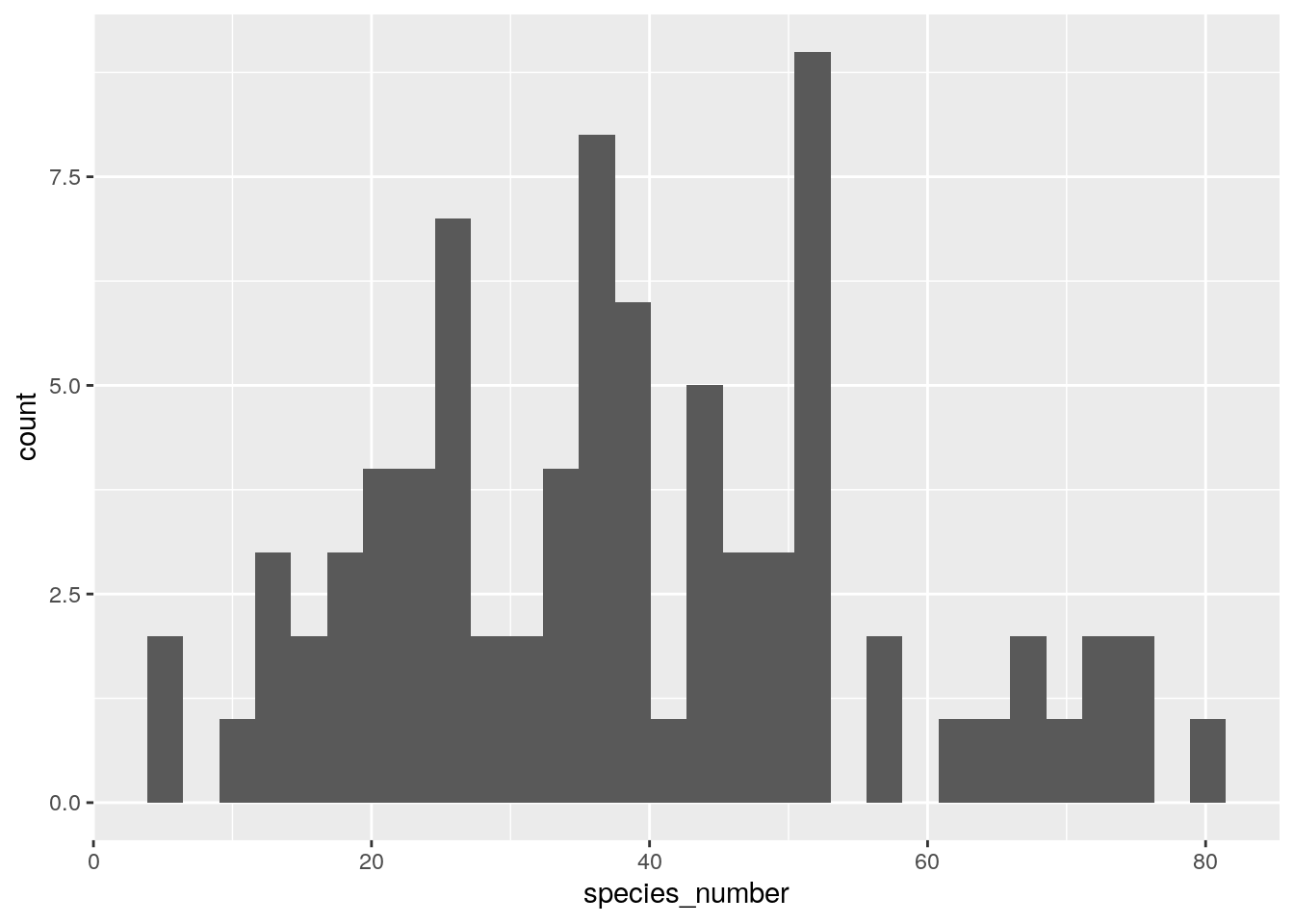
What about the relationship between the two?
ggplot(data.frame(species_number = rowSums(species66[,-1]>0),
                  abundance = rowSums(species66[,-1])),
       aes(abundance, species_number)) +
  geom_point() +
  geom_smooth(method = "lm", formula = y ~ log(x))
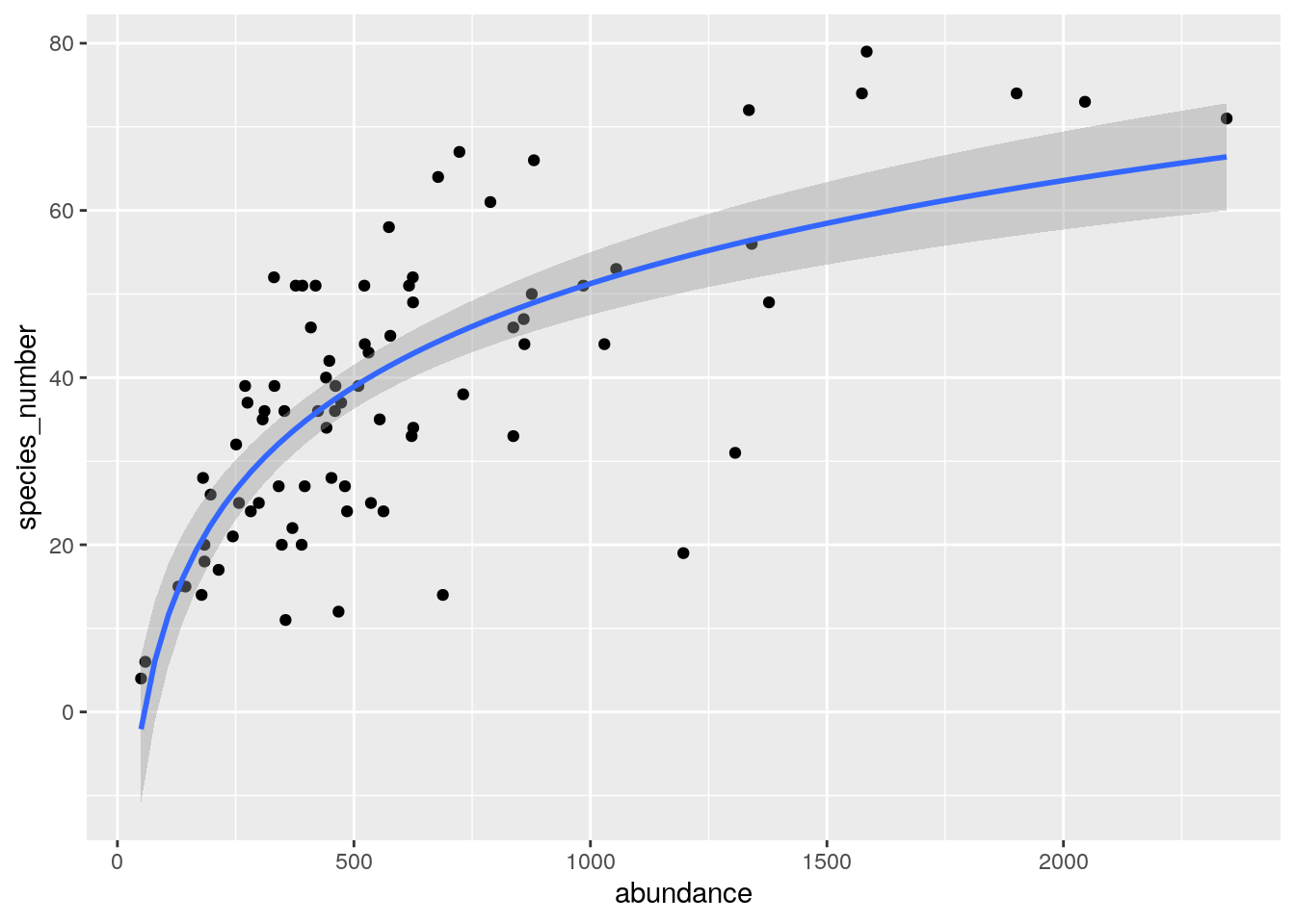
A strong positive relationship. One would usually expect a close relationship between abundance and species number in a vegetation survey, because having more plants in your plot means greater potential to sample more species. E.g. if you only have 10 individuals, the maximum number of species you can sample is 10… In Fynbos, the number of individuals you sample in a set area depends on the vegetation age since fire, with greater numbers in younger plots, because the individuals are smaller.
SIDE NOTE ON SPECIES DIVERSITY MEASURES: This is why I have been referring to species number and not species richness. Species richness, when one looks across all taxonomic groups that use the term, is typically defined as the number of species encountered for a given number of individuals sampled. This accounts for any differences in the amount of effort invested in each sampling event (e.g. trawl netting, mist netting, aerial counts, etc).
It is only when working with sedentary organisms like plants that we typically sample per unit area, in which case we are actually sampling species density and NOT species richness. While useful, species density has different properties to species richness that we should always bear in mind - e.g. species density typically declines with the size of the organism sampled, which depends on the kind of organism (tree vs grass) or the age of the organism (seedling vs adult). One can estimate species richness from vegetation plot data, but that requires having counts of the number of individuals and estimating the average number of species one samples for a given number of individuals. I highly recommend you read Gotelli and Colwell 2001. Ecology Letters if you are ever working with diversity data.
Comparison between surveys
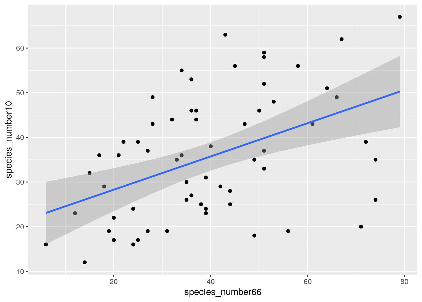
So let’s have a look at the change in diversity within sites between surveys. We can use the same code as above, just plotting the species counts from the one year against the other.
ggplot(data.frame(species_number66 = rowSums(species66[,-1]>0),
                  species_number10 = rowSums(species10[,-1]>0)),
       aes(species_number66, species_number10)) +
  geom_point() +
  geom_smooth(method = "lm")
## Error in data.frame(species_number66 = rowSums(species66[, -1] > 0), species_number10 = rowSums(species10[, : arguments imply differing number of rows: 81, 63
Oh dear! The number of plots surveyed in each year was different for some reason. This is where the plot numbers come in. We need to make sure we’re comparing the same plots. First, we need to see what plot numbers are common between years.
(plots <- intersect(species66$...1, species10$...1))
##  [1] "CP_1"  "CP_10" "CP_12" "CP_13" "CP_14" "CP_15" "CP_16" "CP_17" "CP_18"
## [10] "CP_19" "CP_2"  "CP_21" "CP_22" "CP_27" "CP_28" "CP_29" "CP_3"  "CP_31"
## [19] "CP_34" "CP_36" "CP_37" "CP_38" "CP_39" "CP_4"  "CP_40" "CP_42" "CP_44"
## [28] "CP_45" "CP_46" "CP_47" "CP_48" "CP_49" "CP_50" "CP_55" "CP_56" "CP_57"
## [37] "CP_58" "CP_59" "CP_61" "CP_62" "CP_63" "CP_64" "CP_65" "CP_66" "CP_67"
## [46] "CP_70" "CP_71" "CP_72" "CP_73" "CP_75" "CP_76" "CP_78" "CP_79" "CP_8"
## [55] "CP_80" "CP_82" "CP_83" "CP_88" "CP_89" "CP_9"  "CP_92" "CP_95" "CP_99"
Note that if you get an error, it may be because you don’t have a column called ‘…1’. This was an automatic name R gave the column. On Mac it may be ‘X__1’. If you get an error, run the code names(species66)[1] to see what it called it on your computer and change the column name in the lines of code above and below. Sorry about that.
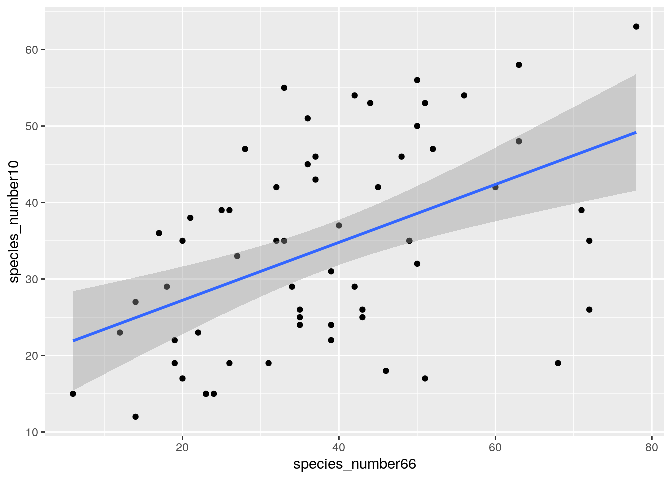
Now we need to extract these “intersect()ing” plots from each survey’s community data matrix, like so
species66c <- species66[which(species66$...1 %in% plots), -1]
species10c <- species10[which(species10$...1 %in% plots), -1]
Now let’s try to look at the change in diversity within sites between surveys again.
ggplot(data.frame(species_number66 = rowSums(species66c>0),
                  species_number10 = rowSums(species10c>0)),
       aes(species_number66, species_number10)) +
  geom_point() +
  geom_smooth(method = "lm")
## `geom_smooth()` using formula 'y ~ x'
Ok, a lot of difference between the two surveys. One thing we haven’t accounted for is the fact that the surveys record all species, but in Fynbos we usually exclude the “seasonally apparent” species like geophytes or annuals and only analyze the data for the “permanently apparent” species. This is because some species are only visible for a few weeks or less, but we only survey the plots once - and not every week for a full year. In this analysis we also want to exclude alien species.
You’ll note that one of the spreadsheets in our dataset is called “excluded_spp”
excel_sheets("pnas.1619014114.sd01.xlsx")
##  [1] "METADATA"           "weather"            "fires"
##  [4] "postfireweather"    "enviroment"         "excluded_spp"
##  [7] "veg1966"            "veg1996"            "veg2010"
## [10] "traits"             "speciesclimatedata"
We need to read these in…
excludes <- read_excel("pnas.1619014114.sd01.xlsx", sheet = "excluded_spp")
## New names:
## * `` -> ...1
head(excludes)
## # A tibble: 6 x 2
##    ...1 x
##   <dbl> <chr>
## 1     1 Acacia saligna
## 2     2 Adenocline pauciflora
## 3     3 Agapanthus walshii
## 4     4 Albuca flaccida
## 5     5 Albuca juncifolia
## 6     6 Annesorhiza altiscapa
…and cut them out of our community data matrices, and plot again
species66c <- species66c[, -which(colnames(species66c) %in% excludes$x)]
species10c <- species10c[, -which(colnames(species10c) %in% excludes$x)]

ggplot(data.frame(species_number66 = rowSums(species66c>0),
                  species_number10 = rowSums(species10c>0)),
       aes(species_number66, species_number10)) +
  geom_point() +
  geom_smooth(method = "lm")
## `geom_smooth()` using formula 'y ~ x'
…very similar. So why the difference among surveys?
Well it could be the differences in post-fire vegetation age and the impacts on the numbers of individuals, and thus species sampled. Let’s look at the relationship between the change in numbers of species and change in vegetation age.
Environmental data
Vegetation age for each plot at the time of each survey is in the enviroment spreadsheet. NOTE that I spelled it incorrectly in the data I submitted to PNAS… Nobody’s perfect…
env <- read_excel("pnas.1619014114.sd01.xlsx", sheet = "enviroment", na = "NA")
## New names:
## * `` -> ...1
head(env)
## # A tibble: 6 x 10
##    ...1  Plot Moisture_class Age1996 Age2010 Age1966 Aliens_max firecount66_10
##   <dbl> <dbl>          <dbl>   <dbl>   <dbl>   <dbl>      <dbl>          <dbl>
## 1     1     1              5      10      10       8          3              3
## 2     2     2              5      10      10       5          1              3
## 3     3     3              5      10      10       7          1              3
## 4     4     4              4      10      24      18          3             NA
## 5     5     8              5      10       3       3          3              2
## 6     6     9              5      10      24       3          2              1
## # … with 2 more variables: firecount66_96 <dbl>, firecount96_10 <dbl>
Ok, first we need to match the plots in the env object to those in the community data matrices. This is a little tricky, because the Plot column in the env object only has numbers, whereas in the community data matrices they were prefixed with “CP_". We’ll have to paste() them in, like so
(env$...1 <- paste("CP_", env$Plot, sep = ""))
##  [1] "CP_1"   "CP_2"   "CP_3"   "CP_4"   "CP_8"   "CP_9"   "CP_10"  "CP_12"
##  [9] "CP_13"  "CP_14"  "CP_15"  "CP_16"  "CP_17"  "CP_18"  "CP_19"  "CP_21"
## [17] "CP_22"  "CP_23"  "CP_24"  "CP_25"  "CP_27"  "CP_28"  "CP_29"  "CP_30"
## [25] "CP_31"  "CP_34"  "CP_36"  "CP_37"  "CP_38"  "CP_39"  "CP_40"  "CP_42"
## [33] "CP_44"  "CP_45"  "CP_46"  "CP_47"  "CP_48"  "CP_49"  "CP_50"  "CP_54"
## [41] "CP_55"  "CP_56"  "CP_57"  "CP_58"  "CP_59"  "CP_60"  "CP_61"  "CP_62"
## [49] "CP_63"  "CP_64"  "CP_65"  "CP_66"  "CP_67"  "CP_68"  "CP_70"  "CP_71"
## [57] "CP_72"  "CP_73"  "CP_74"  "CP_75"  "CP_76"  "CP_78"  "CP_79"  "CP_80"
## [65] "CP_81"  "CP_82"  "CP_83"  "CP_84"  "CP_86"  "CP_87"  "CP_88"  "CP_89"
## [73] "CP_90"  "CP_91"  "CP_92"  "CP_94"  "CP_95"  "CP_97"  "CP_98"  "CP_99"
## [81] "CP_100"
And then join the species10 column names to env. Note that the left_join function retains only the rows that were matched, and it sorts them into the same order as the first object supplied.
Note that you may need to change the ‘…1’ above to whatever your first column of the species10 dataframe is named as mentioned earlier. Otherwise the next line of code returns an empty object and the plotting fails.
env <- left_join(species10[,1], env)
## Joining, by = "...1"
Ok, now we’re ready to plot the change in numbers of species with the change in vegetation age.
ggplot(data.frame(
    change_in_species_number = rowSums(species66c>0) - rowSums(species10c>0),
    change_in_age = env$Age1966 - env$Age2010),
       aes(change_in_species_number, change_in_age)) +
  geom_point() +
  geom_smooth(method = "lm")
## `geom_smooth()` using formula 'y ~ x'
## Warning: Removed 6 rows containing non-finite values (stat_smooth).
## Warning: Removed 6 rows containing missing values (geom_point).
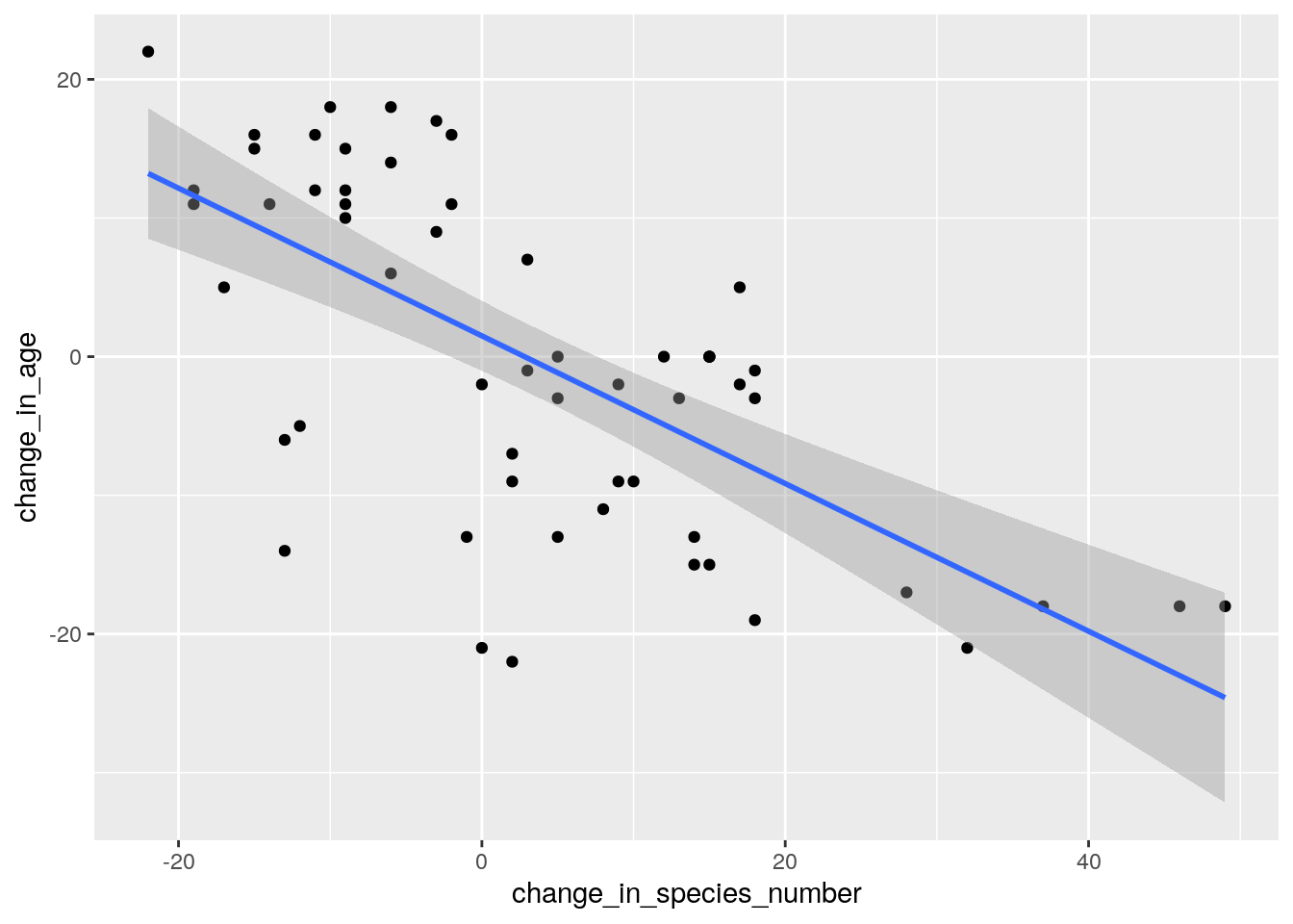
Ignore the error. This is because some the plots don’t have a known vegetation age as they have never burnt on record.
So vegetation age clearly is an issue, with numbers of species declining as the vegetation ages (or increasing after a plot burns).
One approach to deal with this is to “rarefy” the samples. This involves estimating each plot’s expected species richness by randomly sampling a set number of individuals from each community. Again, I highly recommend you read Gotelli and Colwell 2001. Ecology Letters.
In this case we’ll sample 50 individuals, because that is the minimum abundance recorded in our plots.
ggplot(data.frame(species_richness66 = rarefy(x = ceiling(species66c), sample = 50),
                  species_richness10 = rarefy(x = ceiling(species10c), sample = 50)),
       aes(species_richness66, species_richness10)) +
  geom_point() +
  geom_smooth(method = "lm")
## `geom_smooth()` using formula 'y ~ x'
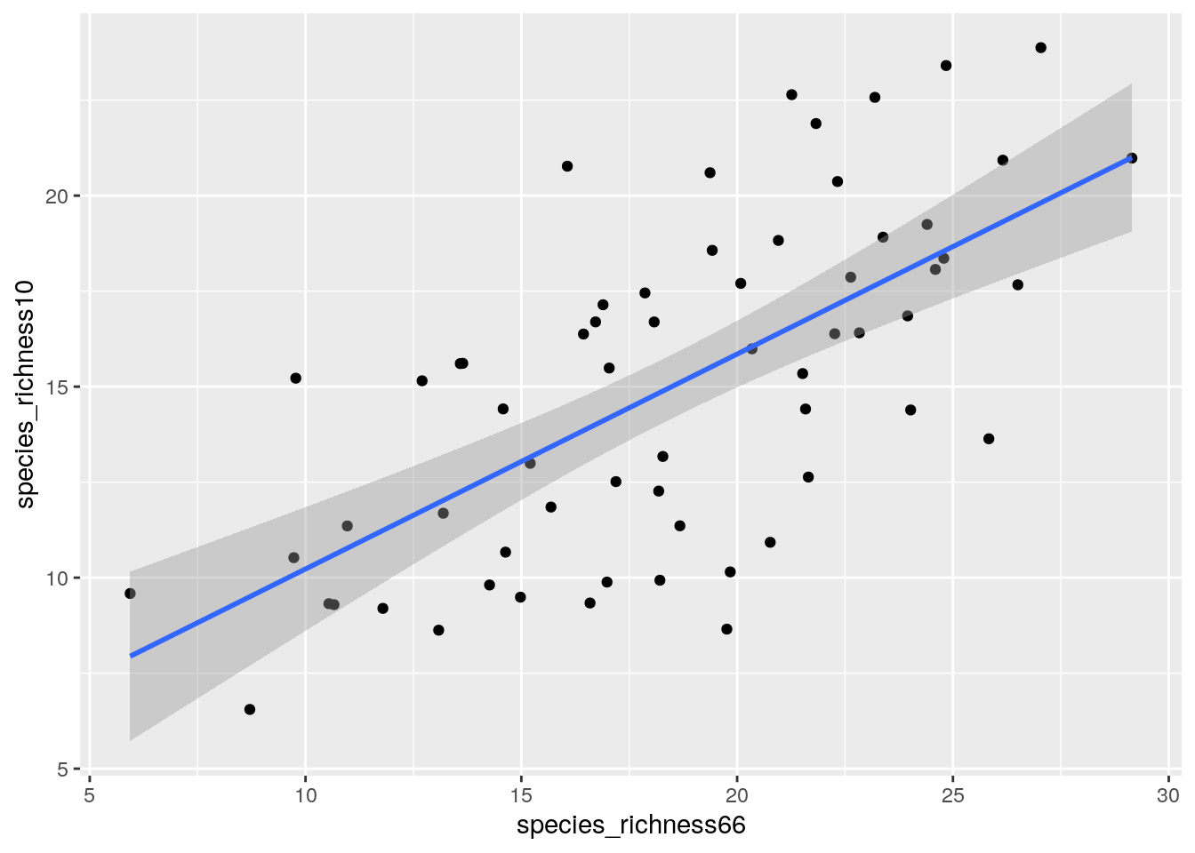
Much more similar… but still some differences. It looks like there may be fewer species in 2010, but this should be revealed by the slope of a regression line. We can get the slope by looking at the summary() of the linear model (lm()),
sr66 <- rarefy(x = ceiling(species66c), sample = 50)
sr10 <- rarefy(x = ceiling(species10c), sample = 50)

summary(lm(sr10 ~ sr66 - 1))
##
## Call:
## lm(formula = sr10 ~ sr66 - 1)
##
## Residuals:
##     Min      1Q  Median      3Q     Max
## -7.0426 -1.9667 -0.1091  2.9906  8.0104
##
## Coefficients:
##      Estimate Std. Error t value Pr(>|t|)
## sr66  0.79423    0.02309    34.4   <2e-16 ***
## ---
## Signif. codes:  0 '***' 0.001 '**' 0.01 '*' 0.05 '.' 0.1 ' ' 1
##
## Residual standard error: 3.51 on 62 degrees of freedom
## Multiple R-squared:  0.9502,	Adjusted R-squared:  0.9494
## F-statistic:  1183 on 1 and 62 DF,  p-value: < 2.2e-16
Note that I forced the intercept to be 0 by adding “-1” to the formula. The interesting thing is that the slope is 0.7942285, which suggests lower species numbers in 2010…
We can also test this using a paired T test
t.test(sr66, sr10, paired = T)
##
## 	Paired t-test
##
## data:  sr66 and sr10
## t = 6.9289, df = 62, p-value = 2.854e-09
## alternative hypothesis: true difference in means is not equal to 0
## 95 percent confidence interval:
##  2.471771 4.476248
## sample estimates:
## mean of the differences
##                3.474009
Yup, there was a significant drop in species numbers between 1966 and 2010, even once we accounted for differences in vegetation age/numbers of individuals. Bear in mind that these results are not necessarily defensible (and do not appear in the paper), because the 1966 “abundance” data is only an estimate made by taking the mid-point of the categorical abundance classes recorded in the original survey. This may well bias the rarefaction results.
The Fourth Corner…
I’m not going to delve into this much, but since one of the biggest topics community ecologists are interested in is the relationship between species’ traits and environmental variables I feel it bears mentioning.
Why is this called “the fourth corner”? I mentioned that analyses of biotic community data typically involve 3 data matrices:
- Species by sites
- Environmental variables by site
- Traits by species
The “fourth corner” is the matrix we have to estimate from the other matrices, because we can’t observe it directly - that of traits by environment.
There are a multitude of methods out there for looking at the fourth corner, and covering this is beyond the scope of this tutorial, but I thought I’d demonstrate one of the simplest approaches - that of comparing the relative dominance of different functional types across different environments.
First we need to read in the trait data, which is the worksheet called traits.
traits <- read_excel("pnas.1619014114.sd01.xlsx", sheet = "traits")
## New names:
## * `` -> ...1
head(traits)
## # A tibble: 6 x 9
##    ...1 species family_GM resprout_postfi…  herb geophyte graminoid low_shrub
##   <dbl> <chr>   <chr>                <dbl> <dbl>    <dbl>     <dbl>     <dbl>
## 1    17 Adenan… RUTACEAE                 0     0        0         0         1
## 2    18 Adenan… RUTACEAE                 0     0        0         0         1
## 3    29 Agatho… RUTACEAE                 1     0        0         0         1
## 4    31 Agatho… RUTACEAE                 1     0        0         0         1
## 5    33 Agatho… RUTACEAE                 0     0        0         0         1
## 6    37 Agatho… RUTACEAE                 1     0        0         0         1
## # … with 1 more variable: tall_shrub <dbl>
You’ll see we have a column called resprout_postfire, which contains information on the postfire regeneration strategy for all species, indicating whether they are killed by fire and have to recruit from seed (0 = obligate seeder) or can persist through fire and resprout from remaining material (1 = sprouter).
First we pull out vectors of the species names matching each regeneration type. I’m sure there’s an easier way, but this at least is relatively transparent.
sprouters <- unlist(na.omit(traits[traits$resprout_postfire == 1,]$species))

seeders <- unlist(na.omit(traits[traits$resprout_postfire == 0,]$species))

sprouters[1:10]
##  [1] "Agathosma bifida"       "Agathosma capensis"     "Agathosma hookeri"
##  [4] "Agathosma imbricata"    "Amphithalea ericifolia" "Aristea africana"
##  [7] "Aristea capitata"       "Aristea glauca"         "Aspalathus linguiloba"
## [10] "Aspalathus microphylla"
Now we use the sets of species names to extract the species counts and abundances for each regeneration type for each plot and bind them into a new dataframe that includes the soil moisture classes. The classes are labelled 1 to 5 representing: 1 = Permanently Wet, 2 = Seasonally Wet, 3 = Seasonally Moist (typically bordering a seasonal wetland with indicators of some influence such as the presence of a few wetland species), 4 = Well-drained (no evidence of topographic influence on soil moisture and likely reliant on mist/fog and rain only), 5 = Dry (essentially class 4 combined with other factors like N aspect and shallow soil that would affect plant water stress).
regen <- data.frame(
  sprouter_spp = as_tibble(species10c>0) %>% select(any_of(sprouters)) %>% rowwise() %>% pmap_dbl(.,sum),
  seeder_spp = as_tibble(species10c>0) %>% select(any_of(seeders)) %>% rowwise() %>% pmap_dbl(.,sum),
  sprouter_abund = as_tibble(species10c) %>% select(any_of(sprouters)) %>% rowwise() %>% pmap_dbl(.,sum),
  seeder_abund = as_tibble(species10c) %>% select(any_of(seeders)) %>% rowwise() %>% pmap_dbl(.,sum),
  soil_moisture = as.factor(env$Moisture_class))
Turn it into tidy (i.e. long format) data for plotting.
regen <- regen %>% pivot_longer(
  cols = c("sprouter_spp", "seeder_spp", "sprouter_abund", "seeder_abund"),
  names_to = c("Regeneration mode", "Variable"),
  names_pattern = "(.*)_(.*)",
  values_to = "Number")

regen
## # A tibble: 252 x 4
##    soil_moisture `Regeneration mode` Variable Number
##    <fct>         <chr>               <chr>     <dbl>
##  1 5             sprouter            spp          19
##  2 5             seeder              spp          31
##  3 5             sprouter            abund       526
##  4 5             seeder              abund      1292
##  5 5             sprouter            spp          19
##  6 5             seeder              spp          27
##  7 5             sprouter            abund       371
##  8 5             seeder              abund      2132
##  9 4             sprouter            spp          19
## 10 4             seeder              spp          29
## # … with 242 more rows
Note the regexpression passed to names_pattern to convert the column names (“sprouter_spp”, “seeder_spp”, “sprouter_abund”, “seeder_abund”) into two columns (“Regeneration mode”, “Variable”) filled with “seeder”/“sprouter” and “spp”/“abund” respectively.
Now we can plot them
pal <- c("#56B4E9", "#CC79A7")#, "#009E73", "#0072B2", "#E69F00") #colourblind palette

ggplot(data = regen, aes(y = `Number`, x = soil_moisture, fill = `Regeneration mode`)) +
  geom_boxplot() +
  facet_wrap(~Variable, scales = "free") +
  theme_bw() +
  theme(axis.text.x = element_text(angle = 90, hjust = 1, vjust = 0.5)) +
  scale_fill_manual(values=rev(pal))
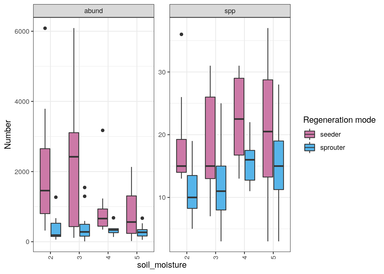
Interestingly, the abundance of seeders is much higher in wetter sites and decreases towards drier sites, while the sprouters show little difference. In contrast, specis counts for both regeneration types increase towards the drier sites. What have I not done (or accounted for) here and how may it confound these results?