Weather stations
One of the biggest challenges of working on global change issues in South Africa is not having easy access to the country’s long-term weather records. One can occasionally access data for research purposes, especially if there’s a student involved, but otherwise our weather service charges a hefty fee for data.
Fortunately, we can access a lot of South Africa’s data through the National Oceanic and Atmospheric Administration of the USA (NOAA) for free here!!!
NOAA serve a massive range of data sets, but the following appear to be the most useful in terms of station data:
BUT WAIT, THERE’S MORE! If you call now, you’ll get this dedicated R package written by the amazing fellows at rOpenSci absolutely free!!!
Here’s a quick demo for using library(rnoaa) below, largely using repurposed and updated code from Scott Chamberlain’s blog posts here and here, and from the package vignette.
DISCLAIMER: We haven’t read the documentation for the datasets and make no guarantee of their accuracy or of the validity of my assumptions when summarizing and presenting the data. This applies to data quality, gaps, units, etc. etc
Let’s get set up…
library("rnoaa")
library("dplyr")
library("reshape2")
library("lawn")
library("leaflet")
library("lubridate")
library("ggplot2")
library("htmltools")
The Integrated Surface Dataset
This dataset “is composed of worldwide surface weather observations from over 35,000 stations”, nominally at hourly resolution. See link above for more details.
Let’s see what stations we can find for South Africa and surrounds?
###Make a bounding box
bbox <- c(16, -35, 34, -22)

###Search the bounding box for stations
out <- isd_stations_search(bbox = bbox)
## using cached file: /home/jasper/.cache/R/noaa_isd/isd_stations.rds## date created (size, mb): 2020-08-02 21:27:15 (0.683)###Have a look at the output
head(out)## # A tibble: 6 x 11
## usaf wban station_name ctry state icao lat lon elev_m begin end
## <chr> <chr> <chr> <chr> <chr> <chr> <dbl> <dbl> <dbl> <dbl> <dbl>
## 1 673080 99999 CHICUALACUALA MZ "" "" -22.1 31.7 453 1.97e7 2.02e7
## 2 673090 99999 DINDIZA-GAZA MZ "" "" -22.1 33.4 102 2.01e7 2.02e7
## 3 673310 99999 MAPULANGUENE-… MZ "" "" -24.5 32.1 151 2.01e7 2.02e7
## 4 673350 99999 XAI XAI MZ "" "FQX… -25.0 33.6 5 1.97e7 2.02e7
## 5 673390 99999 MAPUTO MZ "" "" -26.0 32.6 59 1.95e7 2.02e7
## 6 673410 99999 MAPUTO MZ "" "FQM… -25.9 32.6 44.2 1.97e7 2.02e7Difficult to read a table, so let’s put them on the map.
###Make the popup labels
out$uw <- paste("usaf/wban = ", out$usaf, "/", out$wban, sep = "")
out$period <- paste("years = ", substr(out$begin,1,4), " to ", substr(out$end,1,4), sep = "")
name <- paste(sep = "<br/>", out$station_name, out$period, out$uw)

###Plot the map
leaflet(data = out) %>%
  addTiles() %>%
  addCircleMarkers(label = lapply(name, HTML), radius = 3)
Note that hovering your cursor over the blue circles gives the name of the station, the years operational and the usaf and wban codes required to pull them out of the database (see further down).
There’s also a function for searching for all stations within a specified radius of a point of interest.
out <- isd_stations_search(lat = -34.1, lon = 18.45, radius = 40)
head(out)
## # A tibble: 6 x 12
## usaf wban station_name ctry state icao lat lon elev_m begin end
## <chr> <chr> <chr> <chr> <chr> <chr> <dbl> <dbl> <dbl> <dbl> <dbl>
## 1 6891… 99999 SIMONSTOWN SF "" "" -34.2 18.4 293 1.95e7 1.95e7
## 2 6891… 99999 SLANGKOP SF "" "" -34.2 18.3 8 2.00e7 2.02e7
## 3 6881… 99999 MOLTENO RES… SF "" "" -33.9 18.4 97 2.01e7 2.02e7
## 4 6899… 99999 CT-AWS SF "" "" -34.0 18.6 46 2.00e7 2.02e7
## 5 6881… 99999 CAPE TOWN I… SF "" "FAC… -34.0 18.6 46 1.95e7 2.02e7
## 6 6881… 99999 CAPE TOWN -… SF "" "" -33.9 18.4 2 2.00e7 2.02e7
## # … with 1 more variable: distance <dbl>And if we visualize the area searched…
pt <- lawn::lawn_point(c(18.45, -34.1))
lawn::lawn_buffer(pt, dist = 40) %>% view
Ok, now let’s get a smattering of stations from across the Cape Peninsula that have data for 2019, combine them into one object and plot
###Pull data from online database to local file and then read in
res1 <- isd(usaf=out$usaf[2], wban="99999", year=2019, force = T)
res2 <- isd(usaf=out$usaf[3], wban="99999", year=2019, force = T)
res3 <- isd(usaf=out$usaf[5], wban="99999", year=2019, force = T)
res4 <- isd(usaf=out$usaf[9], wban="99999", year=2019, force = T)

###Combine data into one dataframe
res_all <- bind_rows(res1, res2, res3, res4) #Note that not all stations have all variables and bind_rows() fills empty columns with NAs

###Create a combined date + time column
res_all$date_time <- ymd_hm(
  sprintf("%s %s", as.character(res_all$date), res_all$time)
)

###Convert "temperature" column from codes to numeric and divide by 10 (the data come in tenths of a degree)
res_all$temperature <- as.numeric(substr(res_all$temperature, 2, 5))/10

###Remove the "NA" values, which NOAA code as "999"
res_all$temperature[which(res_all$temperature > 900)] <- NA

###Visualize the data
ggplot(res_all, aes(date_time, temperature)) +
  geom_line() +
  facet_wrap(~usaf_station, scales = "free_x")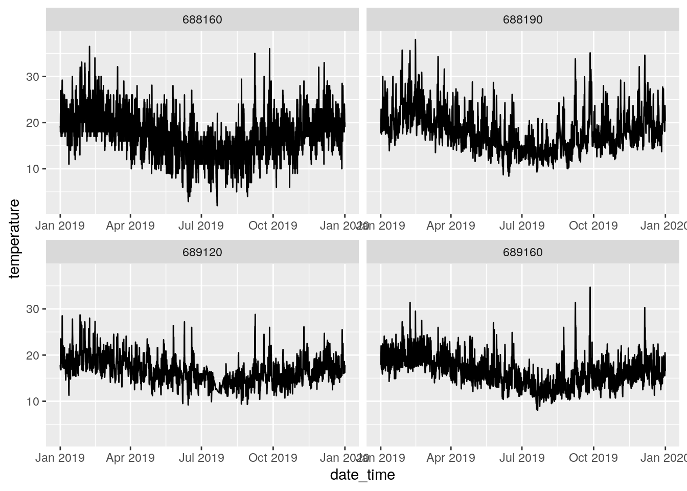
Recall that the ISD dataset is hourly (or mostly 3-hourly in this case), so perhaps better to look at daily max or min temperatures and precipitation?
###Some dodgy cleaning of the rainfall data - CHECK MY ASSUMPTION THAT NA = 0mm RAINFALL
res_all$AA1_depth[is.na(res_all$AA1_depth)] <- 0
res_all$AA1_depth[which(res_all$AA1_depth == 9999)] <- NA
res_all$AA1_depth <- as.numeric(res_all$AA1_depth)

res_all$date <- as.Date(res_all$date, format = "%Y%m%d")

###Summarize Tmin, Tmax and Precipitation
dayres <- res_all %>% group_by(usaf_station, date) %>% summarise(tmax = max(temperature, na.rm = T), tmin = min(temperature, na.rm = T), prec = max(AA1_depth, na.rm = T)/10) #note I take max precip and divide by ten, because it seems to be a hourly cumulative sum in tenths of a mm (Check this!)

###Melt and plot
dayres %>% melt(id = c("usaf_station", "date")) %>% ggplot(aes(date, value, colour = usaf_station)) +
  geom_line() +
  facet_wrap(~variable, scales = "free_y")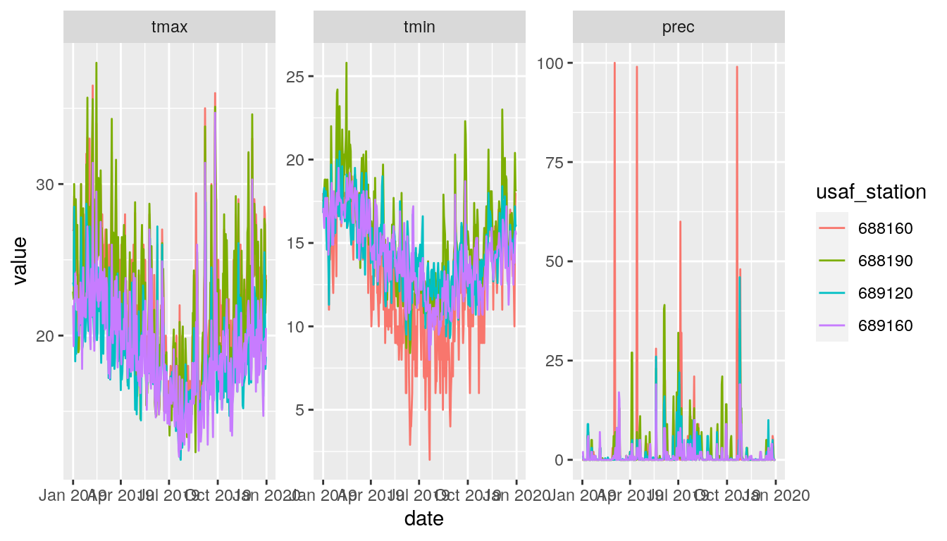
Or monthly…
###Fix dates
res_all$month <- month(res_all$date_time) #note this is all in 2019

###Summarize Tmin, Tmax and Precipitation
monthres <- res_all %>% group_by(usaf_station, month) %>% summarise(tmax = max(temperature, na.rm = T), tmin = min(temperature, na.rm = T), prec = sum(AA1_depth, na.rm = T)/30)

###Melt and plot
monthres %>% melt(id = c("usaf_station", "month")) %>% ggplot(aes(month, value, colour = usaf_station)) +
  geom_line() +
  facet_wrap(~variable, scales = "free_y")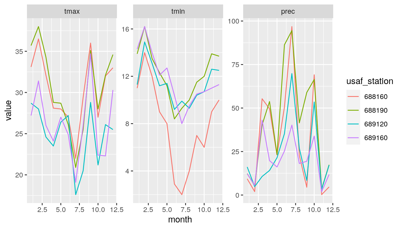
Note that the rnoaa functions save files in a local cache. If you repeat a search, they usually just read in that cache rather than redoing the search and download. Some functions allow you to specify force = TRUE to force a new download, but others don’t. In this case you will need to clear the cache manually. You can find the cache on your machine by calling rappdirs::user_cache_dir("rnoaa/ghcnd").
What if we wanted to look at a longer record? The isd() function only allows us to pull one year at a time so we need to automate using a loop or similar.
We may also be keen to see the names? Or select stations by name rather than usaf/wban codes. You can easily pick your own station names by exploring the interactive map we made above. Then we’ll loop through a few years for each station to get a multi-year record.
Here’s the daily Tmin and Tmax for the period 2013 to 2020 for a few stations around Cape Town.
###Select stations by name and filter
stations <- c("SLANGKOP", "MOLTENO RESERVIOR", "CAPE TOWN INTL", "CAPE POINT")
sout <- filter(out, station_name %in% stations)

###Set date range
yr <- 2013:2020

###Ok, now I'll use 2 nested "for" loops to extract data for all years for each station. "for" loops can often be slower than other approaches like writing functions, but in this case its not a problem because the API call and data download are the slow bit. Using a "for" loop is perhaps easier to follow what I'm doing too.

drtdat <- list() #Make list object to capture outputs (elements will be stations)

#For each station
for (i in 1:nrow(sout)) {

  res <- list() #Make list object to capture interim outputs stations by station (elements will be years)

  #For each year (j), extract the data for station (i)
  for (j in 1:length(yr)) {
    res[[j]] <- tryCatch({
      isd(usaf=sout$usaf[i], wban=sout$wban[i], year=yr[j]) }, error=function(e){cat("ERROR :",conditionMessage(e), "\n")})
  }

  res <- bind_rows(res) #Convert the interim list object into a dataframe
  drtdat[[i]] <- res #Add the dataframe for station i to the output list
}

###Convert output to a dataframe and add the station names
names(drtdat) <- stations
dat <- bind_rows(drtdat)
dat <- right_join(sout[,c("station_name", "usaf")], dat, by = c("usaf"="usaf_station"))

###Create a combined date + time column and year/month/day columns
dat$date_time <- ymd_hm(
  sprintf("%s %s", as.character(dat$date), dat$time)
)
dat$year <- year(dat$date_time) #note this is NOT all in 2019 this time
dat$month <- month(dat$date_time)
dat$day <- month(dat$date_time)
dat$date <- as.Date(dat$date, format = "%Y%m%d")

###Convert "temperature" column from codes to numeric
dat$temperature <- as.numeric(substr(dat$temperature, 2, 5))/10

###Remove the "NA" values, which NOAA code as "999"
dat$temperature[which(dat$temperature > 900)] <- NA

###Some dodgy cleaning of the rainfall data - CHECK MY ASSUMPTION THAT NA = 0mm RAINFALL
dat$AA1_depth[is.na(dat$AA1_depth)] <- 0
dat$AA1_depth[which(dat$AA1_depth == 9999)] <- NA
dat$AA1_depth <- as.numeric(dat$AA1_depth)

###Daily summary of Tmin and Tmax
daydat <- dat %>% group_by(station_name, date) %>% summarise(tmax = max(temperature, na.rm = T), tmin = min(temperature, na.rm = T))

###Melt and plot
daydat %>% melt(id = c("station_name", "date")) %>% ggplot(aes(date, value, colour = variable)) +
  geom_line() +
  facet_wrap(~station_name)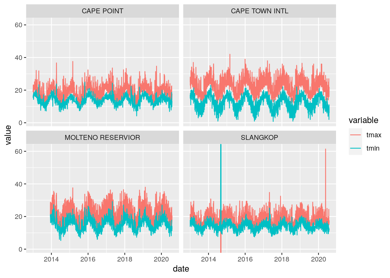
Or precipitation by month?
###Summarize Tmin, Tmax and Precipitation
monthdat <- dat %>% group_by(station_name, year, month) %>% summarise(prec = sum(AA1_depth, na.rm = T)/30)
monthdat$date <- as.Date(paste(monthdat$year, monthdat$month, "01", sep = "/"), format = "%Y/%m/%d")

###Melt and plot
monthdat %>% select(station_name, date, prec) %>% ggplot(aes(date, prec)) +
  geom_line() +
  facet_wrap(~station_name, scales = "free_y")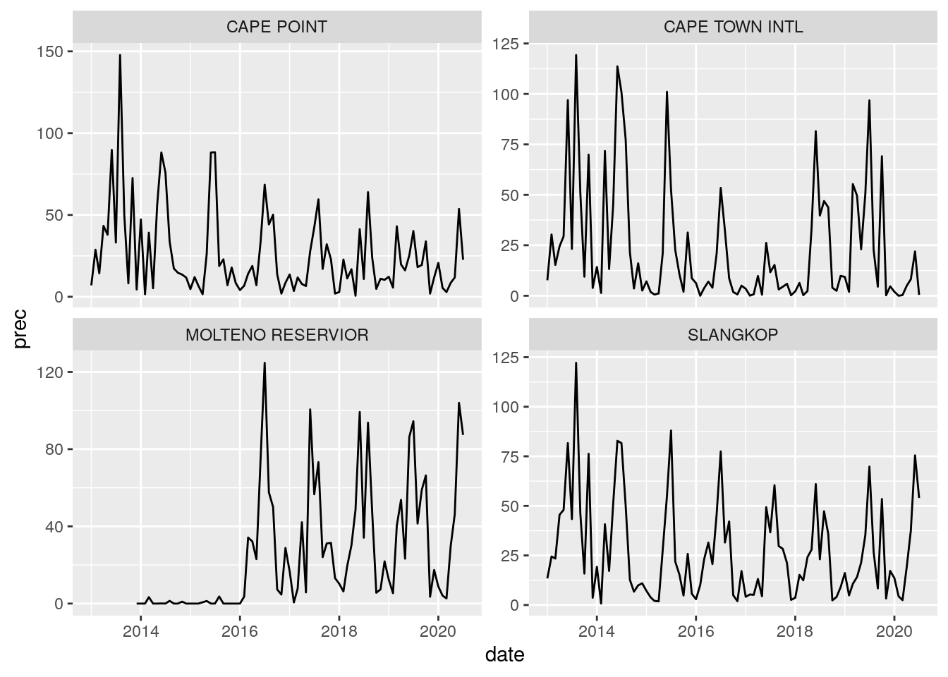
Ok, what about looking at even longer records? Most of South Africa has experienced pretty extreme drought in the past 5 years or so, so let’s pull out a few major cities and towns that give us good coverage of the country.
The Global Historical Climatology Network
Note that the Integrated Surface Dataset (ISD) gives us hourly data, which is overkill for looking at longer records as the dataset gets very large. For this operation it is better to query the Global Historical Climatology Network as described by Menne et al. 2012. CAVEAT: We take no responsibility for the data. Have a look at the paper for details on error corrections, biases, etc.
Let’s have a look at Cape Town International Airport
ct <- meteo_tidy_ghcnd(stationid = "SFM00068816", var = c("TMAX", "TMIN", "PRCP"))

head(ct)
## # A tibble: 6 x 5
## id date prcp tmax tmin
## <chr> <date> <dbl> <dbl> <dbl>
## 1 SFM00068816 1973-06-01 NA NA NA
## 2 SFM00068816 1973-06-02 NA NA NA
## 3 SFM00068816 1973-06-03 NA NA NA
## 4 SFM00068816 1973-06-04 NA NA NA
## 5 SFM00068816 1973-06-05 NA NA NA
## 6 SFM00068816 1973-06-06 NA NA NANote that we had to know the station ID “SFM00068816”. For some reason you can’t query the database of stations using the same method as for the ISD and you have to download the entire list of all ~630 000 global weather stations and query that locally to get the station ID.
station_data <- ghcnd_stations() # Takes a while to run
head(station_data)
## # A tibble: 6 x 11
## id latitude longitude elevation state name gsn_flag wmo_id element
## <chr> <dbl> <dbl> <dbl> <chr> <chr> <chr> <chr> <chr>
## 1 ACW0… 17.1 -61.8 10.1 "" ST J… "" "" TMAX
## 2 ACW0… 17.1 -61.8 10.1 "" ST J… "" "" TMIN
## 3 ACW0… 17.1 -61.8 10.1 "" ST J… "" "" PRCP
## 4 ACW0… 17.1 -61.8 10.1 "" ST J… "" "" SNOW
## 5 ACW0… 17.1 -61.8 10.1 "" ST J… "" "" SNWD
## 6 ACW0… 17.1 -61.8 10.1 "" ST J… "" "" PGTM
## # … with 2 more variables: first_year <int>, last_year <int>You can now query this database using the meteo_nearby_stations() function, which allows you to find all stations within a certain radius of a coordinate or the closest x stations. Here are the closest stations to Cape Point lighthouse.
lat_lon_df <- data.frame(id = "somewhere",
                         latitude = -34.35,
                         longitude = 18.48)
nearby_stations <-  meteo_nearby_stations(lat_lon_df = lat_lon_df,
                    station_data = station_data, radius = 100)

nearby_stations$somewhere
## # A tibble: 23 x 5
## id name latitude longitude distance
## <chr> <chr> <dbl> <dbl> <dbl>
## 1 SF000047220 GROOT CONSTANTIA -34.0 18.4 36.0
## 2 SF000213300 EERSTERIVIER (BOS) -34.0 18.7 41.0
## 3 SF000206890 TABLE.MTN WOODHEAD TUNNEL -34.0 18.4 42.2
## 4 SFM00068816 CAPE TOWN INTL -34.0 18.6 44.3
## 5 SF000207470 TABLE.MTN PLATTEKLIP -34.0 18.4 44.8
## 6 SF000208660 ROYAL OBSERVATORY -33.9 18.5 46.7
## 7 SF000207760 CAPE TOWN FIRE STATION -33.9 18.4 46.9
## 8 SF000207460 TABL.MTN MOLTENO RSV -33.9 18.4 47.0
## 9 SF000210550 CAPE TOWN MAITLAND (CEM) -33.9 18.5 48.0
## 10 SF000216550 STELLENBOSCH (TNK) -33.9 18.9 58.9
## # … with 13 more rowsInteresting… Cape Point lighthouse isn’t on the list, even though it’s a Global Atmospheric Watch station (GAWS) and is in the ISD data. No idea why…
Note that you can also just do a good old text search for the names of a few stations you know. This also allows you to filter by multiple criteria at once, e.g. we can filter for element = PRCP to only get rainfall data. You can use the map we made earlier to get your own list of names, but note that like “CAPE POINT” they’re not all in the GHCND database.
Since most of South Africa has experienced extreme drought in the past few years, perhaps we should pull out and compare the rainfall for a few stations from around the country? In this case we’ve selected a few of the larger towns and cities.
###Select stations by name and filter
stations <- c("CAPE TOWN INTL",
"SPRINGBOK",
"BLOEMFONTEIN AIRPOR",
"PORT ELIZABETH INTL",
"DURBAN INTL",
"JOHANNESBURG INTL")

stas <- station_data %>% filter(element == "PRCP") %>%
  filter(name %in% stations)

stas
## # A tibble: 6 x 11
## id latitude longitude elevation state name gsn_flag wmo_id element
## <chr> <dbl> <dbl> <dbl> <chr> <chr> <chr> <chr> <chr>
## 1 SF00… -29.7 17.9 1007 "" SPRI… "GSN" 68512 PRCP
## 2 SF00… -29.1 26.3 1354 "" BLOE… "GSN" 68442 PRCP
## 3 SFM0… -26.1 28.2 1694. "" JOHA… "" 68368 PRCP
## 4 SFM0… -30.0 31.0 10.1 "" DURB… "" 68588 PRCP
## 5 SFM0… -34.0 18.6 46 "" CAPE… "GSN" 68816 PRCP
## 6 SFM0… -34.0 25.6 68.9 "" PORT… "GSN" 68842 PRCP
## # … with 2 more variables: first_year <int>, last_year <int>Looks like we should be able to compare the period 1980 to 2019 for all stations. Let’s download the data.
dat <- meteo_pull_monitors(stas$id, var = c("TMAX", "TMIN", "PRCP"), date_min = "1980-01-01", date_max = "2019-12-31")

dat[1:5,]
## # A tibble: 5 x 5
## id date prcp tmax tmin
## <chr> <date> <dbl> <dbl> <dbl>
## 1 SF002146700 1980-01-01 0 NA NA
## 2 SF002146700 1980-01-02 0 NA NA
## 3 SF002146700 1980-01-03 0 NA NA
## 4 SF002146700 1980-01-04 0 NA NA
## 5 SF002146700 1980-01-05 0 NA NAOk, now let’s add our station names, summarize by year, and plot.
stas$shortname <- c("SBK", "BFN", "JHB", "DBN", "CPT", "PE")
dat <- left_join(dat, stas[,c("id", "name", "shortname")])
dat$year <- substr(dat$date,1,4)

mdat <- dat %>% group_by(shortname, year) %>% summarise(rain = sum(prcp, na.rm = T)/10) #Get annual totals

mdat$year <- as.numeric(mdat$year)
mdat$rain <- as.numeric(mdat$rain)

###Visualize the data
ggplot(mdat, aes(x = year, y = rain)) +
  geom_line() +
  facet_wrap(~shortname)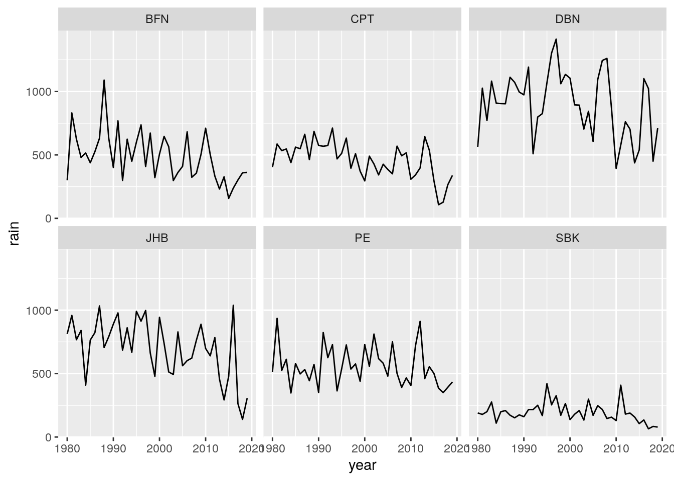
Or something prettier?
###calculate average rainfall and yearly anomalies
ymean <- mdat %>% group_by(shortname) %>% summarise(mean = mean(rain, na.rm = T))
mdat <- left_join(mdat, ymean, by = "shortname")
mdat$positive <- mdat$rain - mdat$mean
mdat$positive[which(mdat$positive<0)] <- 0
mdat$negative <- mdat$rain - mdat$mean
mdat$negative[which(mdat$negative>0)] <- 0

###Plot
ggplot(mdat, aes(x = year)) +
  geom_ribbon(aes(ymin = 0, ymax = positive, fill="positive")) + geom_ribbon(aes(ymin = negative, ymax = 0 ,fill="negative")) +
  scale_fill_manual(name="",values=c("#D6604D", "#4393C3")) +
  facet_grid(shortname ~ ., scales = "free_y") +
  ylab("rainfall anomaly in mm")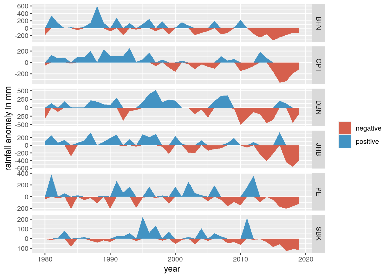
We haven’t dealt with data gaps, data quality verification, etc etc, but this quick and dirty analysis suggests it’s been a pretty dismal decade for South Africa all round…